This (A) markdown shows the descriptive tables and figures, and the “base” plots of actual observed TB diagnoses. We use this base plots in the “analysis” markdown to build up lines showing predictions [including showing our working as going along].
The final (post-analysis) tables and figs are drawn in “b_tableandfig.Rmd”
Load data
library(here)
library(tidyverse)
library(janitor)
library(lubridate)
library(arsenal) # for tableby

acf_start_date <- dmy("01 April 2011")
acf_end_date <- dmy("30 Sep 2014")

# These are the "long" datasets (one row per person with TB)
tb_2009_2018 <- readRDS(file=here("data","tb_2009_2018.rds")) # Each row represents one adult in Blantyre City diagnosed with TB, information on method of TB diagnosis, quarter-year of diagnosis and whether they lived in an ACF or non-ACF area.
tb_2011_2018 <- readRDS(file=here("data","tb_2010_2018.rds")) # Each row represents one adult in Blantyre City diagnosed with TB, but with more information per person than the 2009_2010 file (i.e. includes HIV status, age and sex)
tb_2009_2010 <- readRDS(file=here("data","tb_2009_2010.rds"))
pop <- readRDS(file=here("data","pop.rds")) # Blantyre City adult population by quarter-year and ACF vs. non-ACF area

# These are the "wide" datasets with TB notifications grouped by quarter and with CNR
cnrs_smp_clinic <- readRDS(here("data","cnrs_smp_clinic.rds"))
cnrs_all <- readRDS(here("data","cnrs_all.rds"))  # all form
cnrs_d <- readRDS(here("data","cnrs_d.rds")) # cnrs by method of diagnosis
Figure 1: Map
This is a map of Blantyre. Using “tmap”. Note that shape files are not included in this repo as they have been extremely “fussy” and I have struggled to get them working properly.
library(sf)
library(tmaptools)
library(tmap)
library(OpenStreetMap)


blantyre_city <- sf::st_read(here("data_raw","blantyre_tas.kml")) # rows 1-9 are Blantyre Rural TAs
Reading layer `blantyre_tas' from data source
  `/Users/rachaelburke/Documents/2021_ACF_Blantyre/0_FINAL_ACF/tbacf/data_raw/blantyre_tas.kml'
  using driver `KML'
Simple feature collection with 31 features and 2 fields
Geometry type: MULTIPOLYGON
Dimension:     XY
Bounding box:  xmin: 34.71934 ymin: -16.01844 xmax: 35.13327 ymax: -15.34981
Geodetic CRS:  WGS 84
acf <- blantyre_city[c(9,14:18),]
nonacf <- blantyre_city[c(10:13,19:31),]
clinic <- sf::st_read(here("data_raw","waypoints of facilities and landmarks.shp"))
Reading layer `waypoints of facilities and landmarks' from data source `/Users/rachaelburke/Documents/2021_ACF_Blantyre/0_FINAL_ACF/tbacf/data_raw/waypoints of facilities and landmarks.shp'
  using driver `ESRI Shapefile'
Simple feature collection with 79 features and 12 fields
Geometry type: POINT
Dimension:     XY
Bounding box:  xmin: 34.96957 ymin: -15.85985 xmax: 35.09923 ymax: -15.64464
Geodetic CRS:  WGS 84
clinic <- clinic[c(1:11),]
osm <- read_osm(bb(blantyre_city[c(9:31),], current.projection="wgs84"), ext=1.1, raster=F)
tm_shape(osm) +
tm_rgb() +
tm_shape(nonacf) +
tm_fill(alpha=0.2, col="#46ACC8") +
tm_borders(col="#46ACC8", alpha=0.8) +
tm_shape(acf) +
tm_fill(alpha=0.2, col="#B40F20") +
tm_borders(col="#B40F20", alpha=0.8) +
tm_shape(clinic) +
tm_symbols(size=0.2, shape=15, col="black") +
tm_scale_bar(color.dark = "black") +
tm_compass(position=c("right","top")) +
tm_add_legend(type="fill", col=c("#46ACC8","#B40F20"), labels=c("Non-ACF area","ACF area")) +
tm_add_legend(type="symbol", col="black", shape=15, labels=c("Healthcare clinic")) +
tm_legend(legend.position=c("left","bottom"))

Table 1
Came from data in Dr M Nliwasa’s work / PhD thesis.
Figure 2
cnrs_d <- cnrs_d %>%
  mutate(acfarea_l =
           case_when(acfarea=="b) ACF" ~ "ACF area",
                     acfarea=="a) Non-ACF" ~ "Non-ACF area")) # this is so that the graph gets labelled properly / clearly

diagnosis_method <- ggplot(cnrs_d, aes(x=yq_mid + days(45), y=cnr, fill=diagnosed)) +
  #annotate(geom="rect", xmin=acf_start_date, xmax=acf_end_date, ymin=-Inf, ymax=Inf, alpha=0.4) +
  geom_area(alpha=0.6 , size=.5, colour="black", data=.%>% filter(acfarea=="b) ACF")) +
  geom_area(alpha=0.6 , size=.5, colour="black", data=.%>% filter(acfarea=="a) Non-ACF")) +
  geom_vline(xintercept=acf_start_date, linetype=2) +
  geom_vline(xintercept=acf_end_date, linetype=2) +
  facet_wrap(~acfarea_l) +
  labs(x="Year and quarter",
       y="Case notification rate",
       fill="Method of TB dx") +
  scale_fill_manual(values=c("#46ACC8","#E58601","#E2D200","#B40F20", "#68BB59")) +
  theme_bw()

diagnosis_method

ggsave(plot=diagnosis_method, file=here("figures","Fig2_CNR_by_diagnosis_method.pdf"), width=10, height=7)
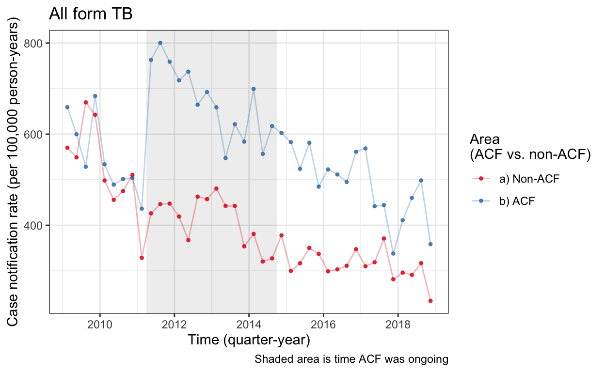
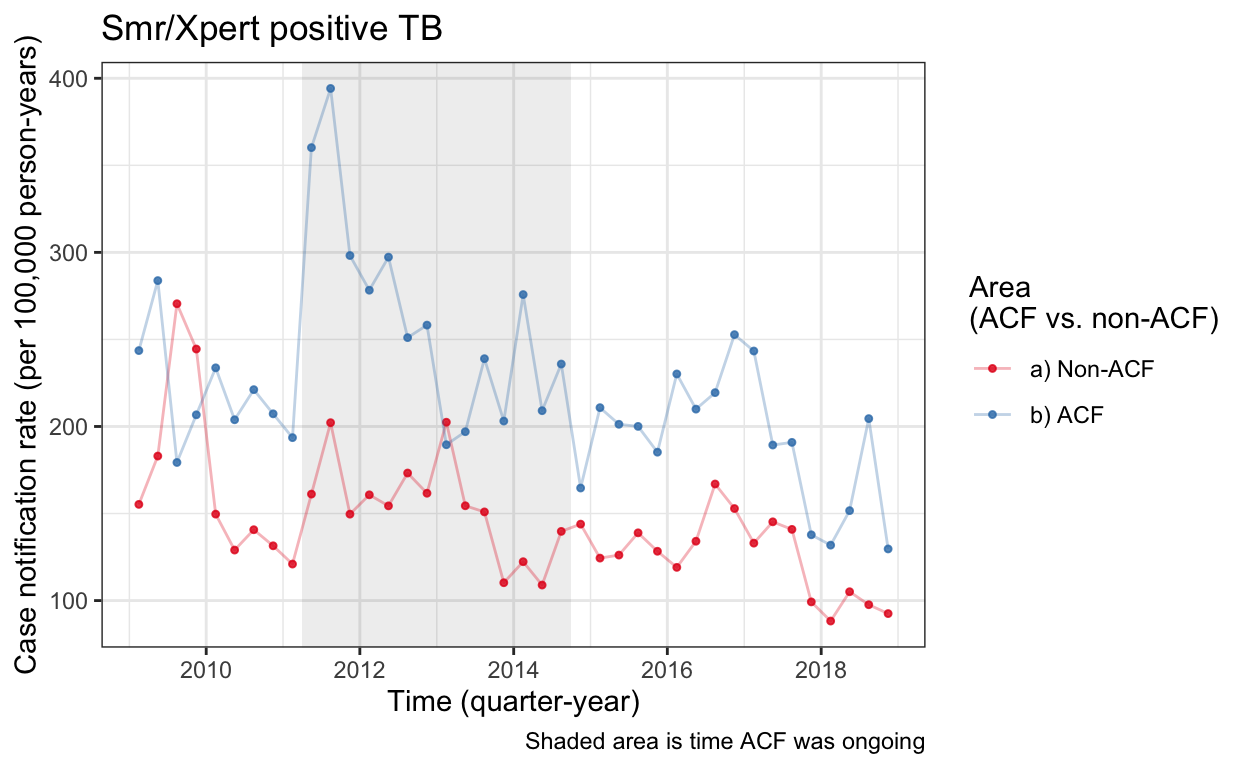
Fig 3 Base plot
This gets built up later with data from “analysis.rmd”. See b_tableandfig for final figure from paper.
plot_fx <- function(df){
ggplot(df) +
  annotate(geom="rect", xmin=acf_start_date, xmax=acf_end_date, ymin=-Inf, ymax=Inf, alpha=0.1) +
  geom_point(aes(x=yq_mid, y=cnr, color=acfarea), shape=20, alpha=0.8) +
  geom_line(aes(y=cnr, x=yq_mid, color=acfarea), alpha=0.3) +
  labs(x="Time (quarter-year)",
       y = "Case notification rate (per 100,000 person-years)",
       color="Area \n(ACF vs. non-ACF)",
       caption="Shaded area is time ACF was ongoing") +
  scale_color_brewer(palette = "Set1") +
  theme_bw()
}

cnr_base_plot_all <- plot_fx(cnrs_all) +
  labs(title="All form TB")
cnr_base_plot_all
cnr_base_plot_micro_clinic <- plot_fx(cnrs_smp_clinic) +
  labs(title="Smr/Xpert positive TB")
cnr_base_plot_micro_clinic
save(cnr_base_plot_micro_clinic, file=here("data/cnr_base_plot_micro_clinic.rdata")) # save both the .rdata object so can re-draw and add
ggsave(plot=cnr_base_plot_micro_clinic, here("figures","cnr_base_plot_micro_clinic.pdf"), width=10, height=7) # and the pdf

save(cnr_base_plot_all, file=here("data/cnr_base_plot_all.rdata")) # save
ggsave(plot=cnr_base_plot_all, file=here("figures","cnr_base_plot_all.pdf"), width=10, height=7)
Numbers quoted in text
Numbers quoted in text.
# A tibble: 2 × 4
# Groups:   yq [1]
  yq         yq_num acfarea    population
  <date>      <dbl> <chr>           <dbl>
1 2011-01-01      8 b) ACF         130173
2 2011-01-01      8 a) Non-ACF     290961
tb_2009_2018 %>% nrow()
[1] 20119tb_2009_2018 %>% tabyl(acf) %>% adorn_totals()
     acf     n   percent
     ACF  7915 0.3934092
 Non-ACF 12204 0.6065908
   Total 20119 1.0000000
tb_2009_2018 %>% tabyl(diagnosed) %>% adorn_totals()
          diagnosed     n     percent
   a) Clinically dx 10705 0.532084100
 b) Smr/cult TB lab  1816 0.090262936
    c) Xpert clinic  1015 0.050449824
      d) Smr clinic  6462 0.321188926
      e) Direct ACF   121 0.006014215
              Total 20119 1.000000000
tb_2009_2018 %>% filter(diagnosed=="d) Smr clinic" | diagnosed=="c) Xpert clinic" | diagnosed=="e) Direct ACF") %>% nrow()
[1] 7598(tb_2009_2018 %>% filter(diagnosed=="d) Smr clinic" | diagnosed=="c) Xpert clinic" | diagnosed=="e) Direct ACF") %>% nrow()) / nrow(tb_2009_2018)
[1] 0.377653[1] 12521(tb_2009_2018 %>% filter(diagnosed=="a) Clinically dx" | diagnosed=="b) Smr/cult TB lab") %>% nrow()) / nrow(tb_2009_2018)
[1] 0.622347tb_2011_2018 %>% tabyl(sex) %>% adorn_totals()
    sex     n   percent
 Female  5813 0.3814805
   Male  9425 0.6185195
  Total 15238 1.0000000
tb_2011_2018 %>% tabyl(ageg) %>% adorn_totals()
  ageg     n    percent
  0-14     0 0.00000000
 15-24  2148 0.14096338
 25-34  5422 0.35582097
 35-44  4548 0.29846437
 45-54  1802 0.11825699
 55-64   783 0.05138470
   65+   535 0.03510959
Total 15238 1.00000000 Min. 1st Qu. Median Mean 3rd Qu. Max.
15.00 26.00 33.00 35.27 41.00 89.00 Min. 1st Qu. Median Mean 3rd Qu. Max.
15.00 29.00 35.00 37.14 43.00 94.00 tb_2011_2018 %>% tabyl(hiv) %>% adorn_totals()
             hiv     n    percent
 a) HIV-negative  4008 0.26302664
 b) HIV-positive 10184 0.66832918
 c) Not recorded  1046 0.06864418
Total 15238 1.00000000# A tibble: 2 × 4
# Groups: yq [1]
yq yq_num acfarea population
<date> <dbl> <chr> <dbl>
1 2009-01-01 0 b) ACF 123155
2 2009-01-01 0 a) Non-ACF 275665# A tibble: 2 × 4
# Groups: yq [1]
yq yq_num acfarea population
<date> <dbl> <chr> <dbl>
1 2018-10-01 39 b) ACF 157331
2 2018-10-01 39 a) Non-ACF 350156# A tibble: 6 × 3
# Groups: acfarea [2]
acfarea acftime cnr
<chr> <fct> <dbl>
1 a) Non-ACF pre-acf 169.
2 a) Non-ACF acf 154.
3 a) Non-ACF post-acf 126.
4 b) ACF pre-acf 219.
5 b) ACF acf 263.
6 b) ACF post-acf 191.# A tibble: 6 × 3
# Groups: acfarea [2]
acfarea acftime cnr
<chr> <fct> <dbl>
1 a) Non-ACF pre-acf 522.
2 a) Non-ACF acf 413.
3 a) Non-ACF post-acf 315.
4 b) ACF pre-acf 548.
5 b) ACF acf 673.
6 b) ACF post-acf 493.tb_2011_2018 %>% nrow()
[1] 15238tb_2011_2018 %>% tabyl(diagnosed)
          diagnosed    n     percent
   a) Clinically dx 7525 0.493831211
 b) Smr/cult TB lab 1816 0.119175745
    c) Xpert clinic 1015 0.066609791
      d) Smr clinic 4761 0.312442578
      e) Direct ACF  121 0.007940675
7525 + 1816
[1] 9341# This is about how many of those who were initially "smear neg" when starting TB treatment were subsequently micro confirmed by culture (by ACF area and ACF time - during ACF vs. post ACF).
# My prefered 'tabyl' options (add totals, percentages)
rmb_tabyl <- function(df) {
df %>% adorn_totals(where="col") %>% adorn_percentages(denominator="row") %>% adorn_pct_formatting(digits=2) %>% adorn_ns()
}
tb_2011_2018 %>%
filter(yq>=dmy("01 April 2011") & yq<dmy("01 Oct 2014")) %>%
filter(diagnosed=="a) Clinically dx" | diagnosed=="b) Smr/cult TB lab") %>%
mutate(diagnosed=as.character(diagnosed)) %>%
tabyl(acfarea,diagnosed) %>% rmb_tabyl()
    acfarea a) Clinically dx b) Smr/cult TB lab          Total
 a) Non-ACF    79.15% (2186)       20.85% (576) 100.00% (2762)
     b) ACF    77.94% (1526)       22.06% (432) 100.00% (1958)
tb_2011_2018 %>%
filter(yq>=dmy("01 April 2011") & yq<dmy("01 Oct 2014")) %>%
mutate(diagnosed=as.character(diagnosed)) %>%
filter(diagnosed=="a) Clinically dx" | diagnosed=="b) Smr/cult TB lab") %>%
tabyl(acfarea, diagnosed) %>% chisq.test(.,tabyl_results=T)
    Pearson's Chi-squared test with Yates' continuity correction

data:  .
X-squared = 0.92627, df = 1, p-value = 0.3358
tb_2009_2018 %>%
filter(acfarea=="b) ACF") %>%
filter(yq>=dmy("01 April 2011")) %>%
mutate(diagnosed=as.character(diagnosed)) %>%
filter(diagnosed=="a) Clinically dx" | diagnosed=="b) Smr/cult TB lab") %>%
tabyl(acftime,diagnosed) %>% rmb_tabyl()
  acftime a) Clinically dx b) Smr/cult TB lab          Total
  pre-acf         -    (0)            -   (0) 100.00%    (0)
      acf    77.94% (1526)       22.06% (432) 100.00% (1958)
 post-acf    80.18% (1541)       19.82% (381) 100.00% (1922)
tb_2009_2018 %>%
filter(acfarea=="b) ACF") %>%
filter(yq>=dmy("01 April 2011")) %>%
mutate(diagnosed=as.character(diagnosed)) %>%
mutate(acftime=as.character(acftime)) %>%
filter(diagnosed=="a) Clinically dx" | diagnosed=="b) Smr/cult TB lab") %>%
tabyl(acftime,diagnosed) %>% chisq.test()
    Pearson's Chi-squared test with Yates' continuity correction

data:  .
X-squared = 2.8052, df = 1, p-value = 0.09396
S. table
Supplementary table numbers (NB. for publication quality output I have re-done this in a dedicated markdown that I could knit to pdf, code here is to display the values in a less “polished” way).
mycontrols  <- tableby.control(test=FALSE)

# Table 1A is pre-ACF (data collected retrospectively)
labels(tb_2009_2010) <- c(diagnosed = "TB type")

Stab1A <- tableby(acf ~ diagnosed, data=tb_2009_2010, control=mycontrols)
summary(Stab1A, title="People with TB 2009-2011.Q1", text=T)
Table: (\#tab:unnamed-chunk-7)People with TB 2009-2011.Q1

|                      | ACF (N=1560) | Non-ACF (N=3321) | Total (N=4881) |
|:---------------------|:------------:|:----------------:|:--------------:|
|TB type               |              |                  |                |
|-  a) Clinically dx   | 936 (60.0%)  |   2244 (67.6%)   |  3180 (65.2%)  |
|-  b) Smr/cult TB lab |   0 (0.0%)   |     0 (0.0%)     |    0 (0.0%)    |
|-  c) Xpert clinic    |   0 (0.0%)   |     0 (0.0%)     |    0 (0.0%)    |
|-  d) Smr clinic      | 624 (40.0%)  |   1077 (32.4%)   |  1701 (34.8%)  |
|-  e) Direct ACF      |   0 (0.0%)   |     0 (0.0%)     |    0 (0.0%)    |
# Table 1B is ACF and post-ACF time (data collected prospectively)
tb_2011_2018b <- tb_2011_2018 %>% mutate(ageg=as.character(ageg)) # this is to get rid of "empty" 0-14 factor
labels(tb_2011_2018b) <- c(ageg = 'Age (years)', sex = "Sex", diagnosed = "TB type", Facility = "Type of Facility", hiv="HIV Status", art = "ART status")
Stab1B <- tableby(acf ~ sex + diagnosed + facility + hiv + art + ageg, data=tb_2011_2018b, control=mycontrols)
summary(Stab1B, title="People with TB 2011.Q2-2018", text=T)
Table: (\#tab:unnamed-chunk-7)People with TB 2011.Q2-2018

|                              | ACF (N=6355) | Non-ACF (N=8883) | Total (N=15238) |
|:-----------------------------|:------------:|:----------------:|:---------------:|
|Sex                           |              |                  |                 |
|-  Female                     | 2467 (38.8%) |   3346 (37.7%)   |  5813 (38.1%)   |
|-  Male                       | 3888 (61.2%) |   5537 (62.3%)   |  9425 (61.9%)   |
|TB type                       |              |                  |                 |
|-  a) Clinically dx           | 3067 (48.3%) |   4458 (50.2%)   |  7525 (49.4%)   |
|-  b) Smr/cult TB lab         | 813 (12.8%)  |   1003 (11.3%)   |  1816 (11.9%)   |
|-  c) Xpert clinic            |  406 (6.4%)  |    609 (6.9%)    |   1015 (6.7%)   |
|-  d) Smr clinic              | 1955 (30.8%) |   2806 (31.6%)   |  4761 (31.2%)   |
|-  e) Direct ACF              |  114 (1.8%)  |     7 (0.1%)     |   121 (0.8%)    |
|facility                      |              |                  |                 |
|-  a) Central hospital        | 2538 (39.9%) |   3683 (41.5%)   |  6221 (40.8%)   |
|-  b) Health centre           | 1892 (29.8%) |   2173 (24.5%)   |  4065 (26.7%)   |
|-  c) Private health facility |  427 (6.7%)  |    619 (7.0%)    |   1046 (6.9%)   |
|-  d) Not recorded            | 1498 (23.6%) |   2408 (27.1%)   |  3906 (25.6%)   |
|HIV Status                    |              |                  |                 |
|-  a) HIV-negative            | 1758 (27.7%) |   2250 (25.3%)   |  4008 (26.3%)   |
|-  b) HIV-positive            | 4170 (65.6%) |   6014 (67.7%)   |  10184 (66.8%)  |
|-  c) Not recorded            |  427 (6.7%)  |    619 (7.0%)    |   1046 (6.9%)   |
|ART status                    |              |                  |                 |
|-  N-Miss                     |     2185     |       2869       |      5054       |
|-  a) Not taking ART          | 932 (22.4%)  |   1298 (21.6%)   |  2230 (21.9%)   |
|-  b) Taking ART              | 3238 (77.6%) |   4716 (78.4%)   |  7954 (78.1%)   |
|Age (years)                   |              |                  |                 |
|-  15-24                      | 884 (13.9%)  |   1264 (14.2%)   |  2148 (14.1%)   |
|-  25-34                      | 2360 (37.1%) |   3062 (34.5%)   |  5422 (35.6%)   |
|-  35-44                      | 1936 (30.5%) |   2612 (29.4%)   |  4548 (29.8%)   |
|-  45-54                      | 662 (10.4%)  |   1140 (12.8%)   |  1802 (11.8%)   |
|-  55-64                      |  306 (4.8%)  |    477 (5.4%)    |   783 (5.1%)    |
|-  65+                        |  207 (3.3%)  |    328 (3.7%)    |   535 (3.5%)    |
Stab <- list(Stab1A, Stab1B)
#write2word(Stab, here("test2.docx"), title="Characteristics of people with TB")