This markdown shows the final figures, incorporating the estimates and their uncertainty. Note that the the CIs for trend here are from “predict” command from the model. Delta method (see “analysis.rmd”) was used to calculate estimates of sum of quarterly diagnosis or mean of quarterly CNRs and it’s CI for tables.
library(tidyverse)
library(data.table)
library(lubridate)
library(here)

acf_start_date <- dmy("01 April 2011")
acf_end_date <- dmy("30 Sep 2014")

# Data - as before (see "setup.rmd")
smp_c <- readRDS(here("data","cnrs_smp_clinic.rds")) %>% filter(acftime!="post-acf") %>% as.data.table()
all_f <- readRDS(here("data","cnrs_all.rds")) %>% filter(acftime!="post-acf") %>% as.data.table() # all form

# Models - as before (see "analysis.rmd")
mod.woc <- readRDS(file=here("data","mod.woc.rds"))
mod.woc.allf <- readRDS(file=here("data","mod.woc.allf.rds"))
mod.wc <- readRDS(file=here("data","mod.wc.rds"))
mod.wc.allf <- readRDS(file=here("data","mod.wc.allf.rds"))

# Base graphs (to illustrate model predictions / fit to real data as we go)
load(here("data/cnr_base_plot_micro_clinic.rdata"))
load(here("data/cnr_base_plot_all.rdata"))

t1 <- smp_c[acftime=='acf',min(yq_num)] # t1 = START of ACF
t2 <- smp_c[acftime=='acf',max(yq_num)] # t2 = END of ACF
T <- t2-t1+1  # plus one because goes from START of first quarter to END of last quarter; this is the TIME (in number of quarters) from ACF starting.
Without control
# This is a dataframe of every level we actually want to make a prediction for to use for calculations
scaffold <- list(
  acftime=c("pre-acf","acf"),
  acfarea=c("b) ACF","a) Non-ACF"),
  yq_num=seq(from=0, to=max(smp_c$yq_num),length.out=200)) %>%
  expand.grid() %>%
  as_tibble() %>%
  arrange(acfarea) %>%
  mutate(population=c(rep(seq(from=min(smp_c[acfarea=="b) ACF"]$population), to=max(smp_c[acfarea=="b) ACF"]$population), length.out = 200), each=2),
  rep(seq(from=min(smp_c[acfarea=="a) Non-ACF"]$population), to=max(smp_c[acfarea=="a) Non-ACF"]$population), length.out = 200), each=2))
) %>%
  arrange(yq_num) %>%
  mutate(yq=rep(seq(from=min(smp_c$yq), to=max(smp_c$yq + months(3)), length.out = 200), each=4)) %>%
  as.data.table()

# this function makes preductions from model multiple timepoints (200 points, see yq_num from "scaffold")
predfx <- function(newdata, model){
  int <- predict(model, newdata=newdata, se.fit=T, type="response")
  newdata %>% mutate(pred=int$fit/population * 4e5,
                            pred.low=(int$fit -1.96*int$se.fit)/population * 4e5,
                            pred.high=(int$fit + 1.96*int$se.fit)/population * 4e5)
}

# Make the preductions
pred.woc.smp <- predfx(scaffold[acfarea=="b) ACF"], mod.woc)  %>%
  mutate(r=case_when( # this is the "real" scenario in woc model (the c'fact is to assume acftime==pre-acf throughout)
    acfarea=="b) ACF" & acftime=="pre-acf" & yq<=acf_start_date ~ T,
    acfarea=="b) ACF" & acftime=="acf" & yq>=acf_start_date & yq<=acf_end_date  ~ T))

pred.woc.allf <- predfx(scaffold[acfarea=="b) ACF"], mod.woc.allf)  %>%
  mutate(r=case_when( # this is the "real" scenario in woc model (the c'fact is to assume acftime==pre-acf throughout)
    acfarea=="b) ACF" & acftime=="pre-acf" & yq<=acf_start_date ~ T,
    acfarea=="b) ACF" & acftime=="acf" & yq>=acf_start_date & yq<=acf_end_date  ~ T))
And plot the graph
fig3a_woc <- cnr_base_plot_micro_clinic +
  geom_line(aes(x=yq, y=pred, linetype="c'factual", color="b) ACF"), data=pred.woc.smp %>% filter(acfarea=="b) ACF", acftime=="pre-acf")) +
  geom_ribbon(aes(x=yq, ymin=pred.low, ymax=pred.high, fill="b) ACF"), alpha=0.1, data=pred.woc.smp %>% filter(acfarea=="b) ACF", acftime=="pre-acf")) +
    geom_line(aes(x=yq, y=pred, linetype="observed", color="b) ACF"), data=pred.woc.smp %>% filter(r==T)) +
  geom_ribbon(aes(x=yq, ymin=pred.low, ymax=pred.high, fill="b) ACF"), alpha=0.1, data=pred.woc.smp %>% filter(r==T)) +
  scale_linetype_manual(values=c(2,1)) +
  scale_color_manual(values=c("#46ACC8","#B40F20","#E58601")) +
  labs(color="Model A", caption="", title="") +
  ylab("CNR: Facility micro. confirmed TB") +
  guides(linetype=F, fill=F) +
  ylim(c(0,420))

fig3a_woc
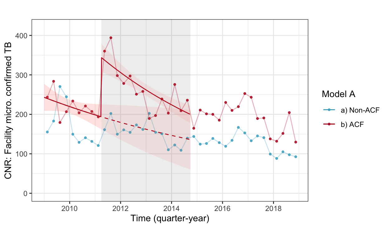
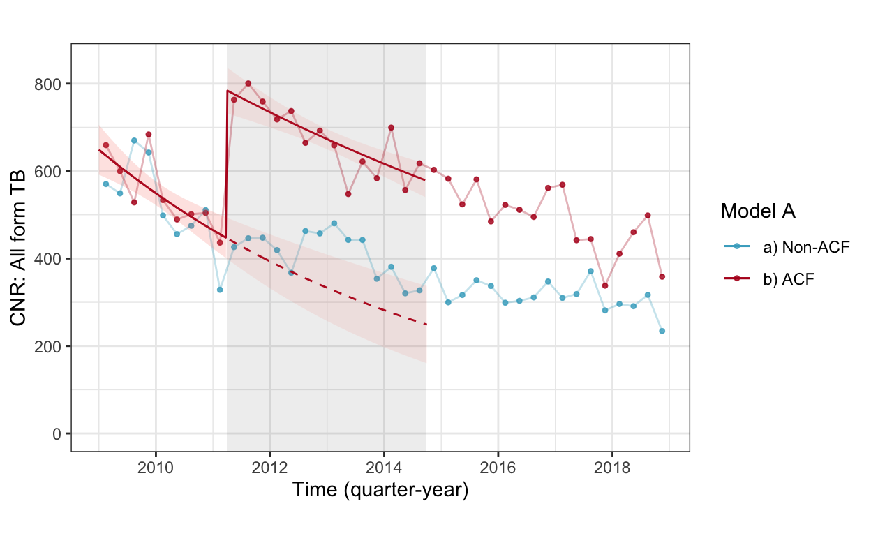
fig3b_woc <- cnr_base_plot_all +
  geom_line(aes(x=yq, y=pred, linetype="c'factual", color="b) ACF"), data=pred.woc.allf %>% filter(acfarea=="b) ACF", acftime=="pre-acf")) +
  geom_ribbon(aes(x=yq, ymin=pred.low, ymax=pred.high, fill="b) ACF"), alpha=0.1, data=pred.woc.allf %>% filter(acfarea=="b) ACF", acftime=="pre-acf")) +
    geom_line(aes(x=yq, y=pred, linetype="observed", color="b) ACF"), data=pred.woc.allf %>% filter(r==T)) +
  geom_ribbon(aes(x=yq, ymin=pred.low, ymax=pred.high, fill="b) ACF"), alpha=0.1, data=pred.woc.allf %>% filter(r==T)) +
  scale_linetype_manual(values=c(2,1)) +
  scale_color_manual(values=c("#46ACC8","#B40F20","#E58601")) +
    labs(color="Model A", caption="", title="") +
  ylab("CNR: All form TB") +
  guides(linetype=F, fill=F) +
  ylim(c(0,850))

fig3b_woc
And with control group
# com=0 is non-ACF
tz <- seq(from=0, to=23, by=0.1)
pop <-c(rep(seq(from=min(smp_c[acfarea=="a) Non-ACF"]$population), to=max(smp_c[acfarea=="a) Non-ACF"]$population), length.out = length(tz)), each=16),
  rep(seq(from=min(smp_c[acfarea=="b) ACF"]$population), to=max(smp_c[acfarea=="b) ACF"]$population), length.out = length(tz)), each=16))
yq <- rep(seq(from=min(smp_c$yq), to=max(smp_c$yq + months(3)), length.out = length(tz)), each=32)


scaffold2 <- list(com=c(0,1),
                  It=c(0,1),
                  tz=tz,
                  Itc=c(0,1),
                  Ittzc=c(0,1),
                  Ittz=c(0,1)) %>%
  expand.grid() %>% as_tibble() %>%
  mutate(Ittzc=Ittzc*tz) %>%
  mutate(Ittz=Ittz*tz) %>%
  arrange(com) %>%
  mutate(population=pop) %>%
  arrange(tz) %>%
  mutate(yq=yq)

pred.wc.smp <- predfx(scaffold2, mod.wc)
pred.wc.allf <- predfx(scaffold2, mod.wc.allf)

whichiswhich <- function(df){
  df %>% mutate(which=case_when(
    com==1 & tz<t1 & It==0 & Ittz==0 & Itc==0 & Ittzc==0 ~ "r+c",
    com==1 & tz>t1 & It==1 & Ittz>t1 & Itc==1 & Ittzc>t1 ~ "r",
    com==0 & tz<t1 & It==0 & Ittz==0 & Itc==0 & Ittzc==0 ~ "n",
    com==0 & tz>t1 & It==1 & Ittz>t1 & Itc==0 & Ittzc==0 ~ "n",
    com==1 & tz>t1 & It==1 & Ittz>t1 & Itc==0 & Ittzc==0 ~ "c",
    ))
}

pred.wc.smp <- pred.wc.smp %>% whichiswhich()
pred.wc.allf <- pred.wc.allf %>% whichiswhich()

fig3a_wc <- cnr_base_plot_micro_clinic +
  geom_line(aes(x=yq, y=pred, linetype="real", color="b) ACF"), data=pred.wc.smp %>% filter(which=="r" | which=="r+c")) +
  geom_line(aes(x=yq, y=pred, linetype="real", color="a) Non-ACF"), data=pred.wc.smp %>% filter(which=="n")) +
  geom_line(aes(x=yq, y=pred, linetype="c'factual", color="c) c'factual"), data=pred.wc.smp %>% filter(which=="c" | which=="r+c")) +
  geom_ribbon(aes(x=yq, ymin=pred.low, ymax=pred.high, fill="b) ACF"), alpha=0.2, data=pred.wc.smp %>% filter(which=="r" | which=="r+c")) +
  geom_ribbon(aes(x=yq, ymin=pred.low, ymax=pred.high, fill="a) Non-ACF"), alpha=0.2, data=pred.wc.smp %>% filter(which=="n")) +
  geom_ribbon(aes(x=yq, ymin=pred.low, ymax=pred.high, fill="c) c'factual"), alpha=0.2, data=pred.wc.smp %>% filter(which=="c" | which=="r+c")) +
  scale_linetype_manual(values=c(2,1)) +
  scale_color_manual(values=c("#46ACC8","#B40F20","#E58601")) +
  scale_fill_manual(values=c("#46ACC8","#B40F20","#E58601")) +
  labs(color="Model B", caption="", title="") +
  ylab("CNR: Facility micro. confirmed TB") +
  guides(linetype=F, fill=F) +
  ylim(c(0,420))

fig3a_wc
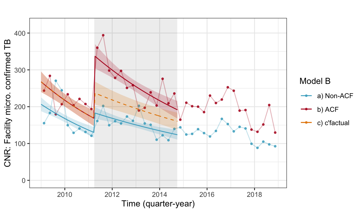
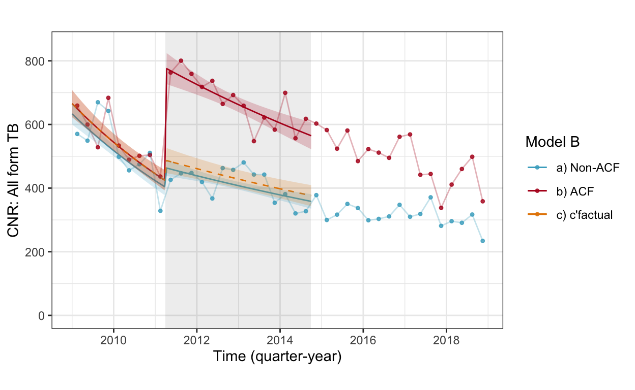
fig3b_wc <- cnr_base_plot_all +
  geom_line(aes(x=yq, y=pred, linetype="real", color="b) ACF"), data=pred.wc.allf %>% filter(which=="r" | which=="r+c")) +
  geom_line(aes(x=yq, y=pred, linetype="real", color="a) Non-ACF"), data=pred.wc.allf %>% filter(which=="n")) +
  geom_line(aes(x=yq, y=pred, linetype="c'factual", color="c) c'factual"), data=pred.wc.allf %>% filter(which=="c" | which=="r+c")) +
  geom_ribbon(aes(x=yq, ymin=pred.low, ymax=pred.high, fill="b) ACF"), alpha=0.2, data=pred.wc.allf %>% filter(which=="r" | which=="r+c")) +
  geom_ribbon(aes(x=yq, ymin=pred.low, ymax=pred.high, fill="a) Non-ACF"), alpha=0.2, data=pred.wc.allf %>% filter(which=="n")) +
  geom_ribbon(aes(x=yq, ymin=pred.low, ymax=pred.high, fill="c) c'factual"), alpha=0.2, data=pred.wc.allf %>% filter(which=="c" | which=="r+c")) +
  scale_linetype_manual(values=c(2,1)) +
  scale_color_manual(values=c("#46ACC8","#B40F20","#E58601")) +
  scale_fill_manual(values=c("#46ACC8","#B40F20","#E58601")) +
  labs(color="Model B", caption="", title="") +
  ylab("CNR: All form TB") +
  guides(linetype=F, fill=F) +
  ylim(c(0,850))

fig3b_wc
Save these four
ggsave(plot=fig3a_woc, here("figures","fig3a_woc.pdf"), width=7, height=4)
ggsave(plot=fig3b_woc, here("figures","fig3b_woc.pdf"),width=7, height=4)
ggsave(plot=fig3a_wc, here("figures","fig3a_wc.pdf"), width=7, height=4)
ggsave(plot=fig3b_wc, here("figures","fig3b_wc.pdf"), width=7, height=4)

saveRDS(fig3a_woc, here("data","fig3a_woc.rdata"))
saveRDS(fig3b_woc, here("data","fig3b_woc.rdata"))
saveRDS(fig3a_wc, here("data","fig3a_wc.rdata"))
saveRDS(fig3b_wc, here("data","fig3b_wc.rdata"))