What is the significance of chosen inflection point?
library(MASS)
library(here)
library(tidyverse)
library(lubridate)
library(zoo)

tb_data_group <- read_csv(here("data","tb_data_group.csv"))
covid_date_m <- dmy("01 April 2020") # date of COVID starting (whole month)
covid_month_num <- 47

load(here("data/Pop_Age_Sex_HIV.rdata")) # Blantyre census data disaggregated by age and sex (from world population prospects and modified by CCK)
cens <- PopQ %>%
  mutate(year_q=paste0(Year,":",Q)) %>%
  mutate(yq=yq(year_q)) # yq is a date with 1st day of each quarter

age_levels_10 <- c("0-14","15-24", "25-34", "35-44", "45-54", "55-64", "65+")

tb_data <- tb_data_group %>% uncount(n) %>% mutate(month=dmy(month)) %>% mutate(fac=factor(fac),
                                                                                sex = factor(sex),
                                                                                hiv = factor(hiv))

cens_10yr <- cens %>% mutate(age_gp=case_when(
  Age=="[0,4)" ~ "0-14",
  Age=="[5,9)" ~ "0-14",
  Age=="[10,14)" ~ "0-14",
  Age=="[15,19)" ~ "15-24",
  Age=="[20,24)" ~ "15-24",
  Age=="[25,29)" ~ "25-34",
  Age=="[30,34)" ~ "25-34",
  Age=="[35,39)" ~ "35-44",
  Age=="[40,44)" ~ "35-44",
  Age=="[45,49)" ~ "45-54",
  Age=="[50,54)" ~ "45-54",
  Age=="[55,59)" ~ "55-64",
  Age=="[60,64)" ~ "55-64",
  Age=="[60,64)" ~ "55-64",
  Age=="[65,69)" ~ "65+",
  Age=="[70,74)" ~ "65+",
  Age=="[75, )" ~ "65+"
)) %>%
  group_by(yq, age_gp, Sex) %>%
  summarise(pop=sum(Population))

cens_all <- cens %>%
  group_by(yq) %>%
  summarise(pop=sum(Population)) %>%
  mutate(`0`=pop,  # so this is a slightly hacky way to get population demoninators for each month (the quarter denominator gets repeated the same three times, not ideal, but it doesn't make any difference.  For plotting the graph - where CNR is a continous variable, I interpolate population to avoid zigzags)
         `1`=pop,
         `2`=pop) %>%
  pivot_longer(c(`0`,`1`,`2`),names_to="m") %>%
  mutate(m=as.numeric(m)) %>%
  mutate(month=yq+months(m))

# then this is dataframe lumping all cases togehter
all <- tb_data %>%
  group_by(month) %>%
  summarise(cases=n()) %>% #generates cases per month
  ungroup() %>%
  mutate(covid = if_else(month >= covid_date_m, 1L,0L)) %>%
  arrange(month) %>%
  mutate(month_num = 1:n()) %>% #create a month_num variable to use in model (rather than actual date, so coefficients make sense)
  left_join(cens_all) %>%
  mutate(cnr=(cases/pop)*100000*12) # x12 to get annualised CNRs (NB. children included in both denominator and numerator here)
m <-glm.nb(cases ~ month_num + offset(log(pop)), data=all) # model without specifying COVID time
res <- residuals(m)
res_df <- res %>% as_tibble_col(column_name="res") %>% cbind(all$month_num) %>% rename(month_num=`all$month_num`)
res_df <- res_df %>% mutate(movingav=zoo::rollmean(res,k=5, na.pad=T, align="left"))
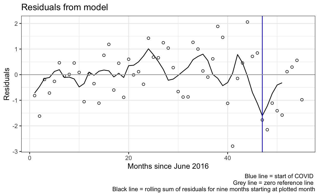
ggplot(res_df) +
geom_point(aes(x=month_num, y=res),shape=1) +
geom_line(aes(x=month_num, y=movingav)) +
geom_vline(aes(xintercept=covid_month_num), color="blue") + # add a line at covid_month_num
geom_hline(aes(yintercept=0), color="darkgrey") + # add a zero line
labs(title="Residuals from model",
caption="Blue line = start of COVID \n Grey line = zero reference line \n Black line = rolling sum of residuals for nine months starting at plotted month") +
ylab("Residuals") +
xlab("Months since June 2016") +
theme_bw()
## last 9 are 'covid'
ressum <- sum(rev(res)[1:9]) #test statistic: sum of residuals

N <- 1e6 #number of perms: I tried up to 1e6 (bit slow, but stable P)
permute.vec <- function(X) X[sample(length(X),replace = FALSE)]
## permute.vec <- function(X) X #for testing
permute.vec(res) #test
          53           44           18           45           30
 0.296485714  2.057099211  0.447358892  0.714035154 -0.659526588
          17           36            8           33           32
-0.600903283 -0.096255482  0.010083410  1.263587570 -0.868022538
          28           43           34           47           25
 1.038083155  0.456478153  0.999874178 -1.768416420  0.683105486
           6           13            7           11           38
 0.464648766 -0.350220488 -0.046408481 -1.055558924  1.884665153
           4           12           15           49           55
-0.717101405  0.027924020  0.756811030 -1.111760550 -0.979214352
          19           31            5           22           24
-0.884675966 -0.874028706 -0.260904523  0.115737346  1.424002604
           2           26           37           46           23
-1.617560992  0.658967896  0.617934234  0.845505178 -0.374750290
          20           40            1            3           21
 0.602567186 -1.119096154 -0.818146182 -0.187565884 -0.008955361
          48           50           42           41           14
-2.150209970 -1.408940975 -0.147192969 -2.791492635 -1.112986129
          29           27            9           54           51
 0.273721355  1.247464391  0.455950858  0.559682350 -1.579115609
          39           35           10           52           16
 1.456342275  0.145075331  0.088058979  0.117361206  1.183886648
resmat <- matrix(res,nrow=N,ncol=length(res),byrow = TRUE)
resmat <- apply(resmat,1,permute.vec)
resmat <- t(resmat) #each row a permutation of resds
last9 <- length(res) - 1:9 + 1 #indices of last 9 columns
resmat <- resmat[,last9] #restrict to last 9 columns
res.dist <- rowSums(resmat) #distribution of statistic for perms
length(res.dist)
[1] 1000000hist(res.dist)

summary(res.dist)
    Min.  1st Qu.   Median     Mean  3rd Qu.     Max.
-13.1095 -2.3350 -0.3969 -0.4416 1.4922 10.5439 mean(res.dist<ressum) #P value~0.004 (what quantile is obs'd test stat?)
[1] 0.003678## re-run a few times to ensure accurate as quoted
## now consider other windows of length 9 when a drop may have happened:
ressums <- list() #window locations 1 to just shy of last 9
for(i in 1:(1+length(res)-2*9))
ressums[[i]] <- sum(res[seq(from=i,length.out = 9)])
Pvals <- lapply(ressums,function(x) mean(res.dist<x)) #as above: quantile
Pvals <- unlist(Pvals)
Pvals
 [1] 0.209867 0.310922 0.382698 0.411663 0.462460 0.347372 0.385640
 [8] 0.556247 0.470577 0.469405 0.338378 0.565622 0.560344 0.625389
[15] 0.719920 0.795044 0.739842 0.864833 0.919005 0.984102 0.977974
[22] 0.960608 0.916414 0.884439 0.872608 0.895410 0.856907 0.718173
[29] 0.665456 0.843859 0.964462 0.956427 0.839226 0.684414 0.612740
[36] 0.835369 0.898664 0.912789all(Pvals>0.05) #TRUE - no others are significant
[1] TRUE