Code

Code for our Interrupted Time Series Analysis

1. Load packages and data

# Packages
library(MASS, exclude="select") # for glm.nb
library(tidyverse)
library(readxl)
library(lubridate)
library(broom)
library(here)
library(gt) # make tables loook nice
library(stringr)
library(tsModel) #for including harmonic fx for seasonality
library(boot)
library(mice)
library(janitor) #for tabyl
library(zoo) #for na.approx (interpolate values of population when month treated continuously)

# Load the data

tb_data_group <- read_csv(here("data","tb_data_group.csv"))

load(here("data/Pop_Age_Sex_HIV.rdata")) # Blantyre census data disaggregated by age and sex (from world population prospects and modified by CCK)
cens <- PopQ %>%
  mutate(year_q=paste0(Year,":",Q)) %>%
  mutate(yq=yq(year_q)) # yq is a date with 1st day of each quarter

age_levels_10 <- c("0-14","15-24", "25-34", "35-44", "45-54", "55-64", "65+")
covid_date_m <- dmy("01 Apr 2020") # date of COVID starting (whole month)

Define some functions for use later

# These functions takes a model and makes predictions and puts them into a dataframe (including counterfactual no-COVID)

# The first functions give a df containing one observation per month and predictions for all the levels contained in data plus a counterfactual "no COVID" time.  This is used for calculating expected cumlative numbers of TB cases / CNR (particularly in counterfactual months).

# In second function month is not integer-coded but is continuous -- this is for plotting the graphs so that there is an instaneous effect of COVID (with integer-coded months the drop between March and April was a diagonal line on the graph connecting March and April 2020, which didn't make sense as we'd modelled an instaneneous drop)

model2pred_pop <- function(df,m){ #incorporating a population term to give CNRs

scaffold_df <- all %>% 
  select(month_num,covid) %>% 
  tidyr::expand(month_num,covid) %>% #makes predictions over every level that exists in the data
  left_join(all%>%select(month,month_num,pop))

pred_obj <- predict(m, type="link", newdata=scaffold_df, se.fit=T)

df1 <- scaffold_df %>%
  left_join(all) %>%
  rename(cases_actual=cases) %>%
  rename(cnr_actual=cnr) %>%
  mutate(cases_pred=(exp(pred_obj$fit))) %>%
  mutate(cnr_pred=exp(
    pred_obj$fit - log(pop)
  ) * 100000 * 12) %>%
  mutate(cases_low=(exp(pred_obj$fit - 1.96*pred_obj$se.fit))) %>%
  mutate(cases_high=(exp(pred_obj$fit + 1.96*pred_obj$se.fit))) %>%
  mutate(cnr_low=exp(
    (pred_obj$fit - 1.96*pred_obj$se.fit) - log(pop)
    )
    *100000 * 12 ) %>%
  mutate(cnr_high=exp(
    (pred_obj$fit + 1.96*pred_obj$se.fit) - log(pop)
    ) *100000 * 12) %>%
  mutate(cases_se=pred_obj$se.fit) %>%
  mutate(cases_link=pred_obj$fit) #need to have this on link scale to bootstrap later

df2 <- df1 %>%
  mutate(irrelevant=case_when(
    covid==1 & month_num < covid_month_num ~ T,
    TRUE ~ F
  )) %>%
  filter(irrelevant!=T) %>%  #get rid of "COVID"=yes when time is before COVID (irrelevant predictions)
  select(-irrelevant) %>%
  mutate(c_fact=case_when(
        covid==0 & month_num >= covid_month_num ~ T, #create a variable to indicate no-COVID by after COVID-time is counterfactual
        T ~ F
  ))
df2
}

model2pred_pop_continuous <- function(df,m){ #incorporating a population term to give CNRs

seq <- seq(0,1, length=100) %>% tibble() # creates 100 data point between start and end month numbers (i.e. "month num" becomes nearly continuous)

expand_months <- all %>% 
  dplyr::select(month_num,covid) %>% 
  tidyr::expand(month_num,covid, seq$.) %>% # now includes 1000 extra points for each level of covid and month_num
  mutate(month_num=`seq$.` + month_num) %>% # makes a 'continous' variable for month_num (have to keep name month_num so that plotting works as that's the variable name in model)
  select(-`seq$.`)

x <- all %>% select(month_num, month) # I need this to get actual months back, not just month_num

expand_pop <- expand_months %>% 
  left_join(all, by=c("month_num")) %>%
  select(month_num,covid.x, pop) %>%
  rename(covid=covid.x)%>%
  na.approx() %>% # from zoo package, linear interpolation of population between quarters (to match months now being effectively continuous)
  na.locf() %>% 
  as.data.frame() %>%
  left_join(x)

scaffold_df_continuous <- expand_pop

pred_obj <- predict(m, type="link", newdata=scaffold_df_continuous, se.fit=T)

df1 <- scaffold_df_continuous %>%
  left_join(all) %>% # this brings calendar month back but only when COVID=
  rename(cases_actual=cases) %>%
  rename(cnr_actual=cnr) %>%
  mutate(cases_pred=(exp(pred_obj$fit))) %>%
  mutate(cnr_pred=exp(
    pred_obj$fit - log(pop)
  ) * 100000 * 12) %>%
  mutate(cases_low=(exp(pred_obj$fit - 1.96*pred_obj$se.fit))) %>%
  mutate(cases_high=(exp(pred_obj$fit + 1.96*pred_obj$se.fit))) %>%
  mutate(cnr_low=exp(
    (pred_obj$fit - 1.96*pred_obj$se.fit) - log(pop)
    )
    *100000 * 12 ) %>%
  mutate(cnr_high=exp(
    (pred_obj$fit + 1.96*pred_obj$se.fit) - log(pop)
    ) *100000 * 12) %>%
  mutate(cases_se=pred_obj$se.fit) %>%
  mutate(cases_link=pred_obj$fit) #need to have this on link scale to bootstrap later

df2 <- df1 %>%
  mutate(irrelevant=case_when(
    covid==1 & month_num < covid_month_num ~ T,
    TRUE ~ F
  )) %>%
  filter(irrelevant!=T) %>%  #get rid of "COVID"=yes when time is before COVID (irrelevant predictions)
  select(-irrelevant) %>%
  mutate(c_fact=case_when(
        covid==0 & month_num >= covid_month_num ~ T, #create a variable to indicate no-COVID by after COVID-time is counterfactual
        T ~ F
  ))
df2
}


model2pred_by <- function(df,m){ 

scaffold_df <- df %>% 
  dplyr::filter(hiv!="unknown") %>% 
  dplyr::filter(is.na(sex)==F) %>%
  select(month_num,covid,fac,hiv,sex) %>% 
  tidyr::expand(month_num,covid,fac,hiv,sex) %>% #makes predictions over every level
  left_join(by%>%select(month,month_num)%>%distinct())

pred_obj <- predict(m, type="link", newdata=scaffold_df, se.fit=T)

df1 <- scaffold_df %>%
  left_join(df) %>%
  rename(cases_actual=cases) %>%
  mutate(cases_pred=(exp(pred_obj$fit))) %>%
  mutate(cases_low=(exp(pred_obj$fit - 1.96*pred_obj$se.fit))) %>%
  mutate(cases_high=(exp(pred_obj$fit + 1.96*pred_obj$se.fit))) %>%
  mutate(cases_se=pred_obj$se.fit) %>%
  mutate(cases_link=pred_obj$fit) #need to have this on link scale to bootstrap later

df2 <- df1 %>%
  mutate(irrelevant=case_when(
    covid==1 & month_num < covid_month_num ~ T,
    TRUE ~ F
  )) %>%
  filter(irrelevant!=T) %>%  #get rid of "COVID"=yes when time is before COVID (irrelevant predictions)
  select(-irrelevant) %>%
  mutate(c_fact=case_when(
        covid==0 & month_num >= covid_month_num ~ T, 
        T ~ F))
df2
}

model2pred_by_continuous <- function(df,m){ 

  seq <- seq(0,1, length=100) %>% tibble() # creates 100 data point between start and end month numbers (i.e. "month num" becomes nearly continuous)

  expand_months <- df %>% 
  dplyr::select(month_num,covid) %>% 
  tidyr::expand(month_num,covid, seq$.) %>% # now includes 1000 extra points for each level of covid and month_num
  mutate(month_num=`seq$.` + month_num) %>% # makes a 'continous' variable for month_num (have to keep name month_num so that plotting works as that's the variable name in model)
  select(-`seq$.`)
  
  x <- df %>%
  dplyr::filter(hiv!="unknown") %>% 
  dplyr::filter(is.na(sex)==F) 
  
  scaffold_df <- expand_months %>% left_join(x) %>%
  select(month_num,covid,fac,hiv,sex) %>% 
  tidyr::expand(month_num,covid,fac,hiv,sex) %>% #makes predictions over every level
  left_join(by%>%select(month,month_num)%>%distinct())

pred_obj <- predict(m, type="link", newdata=scaffold_df, se.fit=T)

df1 <- scaffold_df %>%
  left_join(df) %>%
  rename(cases_actual=cases) %>%
  mutate(cases_pred=(exp(pred_obj$fit))) %>%
  mutate(cases_low=(exp(pred_obj$fit - 1.96*pred_obj$se.fit))) %>%
  mutate(cases_high=(exp(pred_obj$fit + 1.96*pred_obj$se.fit))) %>%
  mutate(cases_se=pred_obj$se.fit) %>%
  mutate(cases_link=pred_obj$fit) #need to have this on link scale to bootstrap later


df2 <- df1 %>%
  mutate(irrelevant=case_when(
    covid==1 & month_num < covid_month_num ~ T,
    TRUE ~ F
  )) %>%
  filter(irrelevant!=T) %>%  #get rid of "COVID"=yes when time is before COVID (irrelevant predictions)
  select(-irrelevant) %>%
  mutate(c_fact=case_when(
        covid==0 & month_num >= covid_month_num ~ T, 
        T ~ F))
df2
}

2. Get data into required format

NB. “All” is grouped data of total number of TB cases by month.

tb_data <- tb_data_group %>% uncount(n) %>% mutate(month=dmy(month)) %>% mutate(fac=factor(fac),
                                                                                sex = factor(sex),
                                                                                hiv = factor(hiv))

cens_10yr <- cens %>% mutate(age_gp=case_when(
  Age=="[0,4)" ~ "0-14",
  Age=="[5,9)" ~ "0-14",
  Age=="[10,14)" ~ "0-14",
  Age=="[15,19)" ~ "15-24",
  Age=="[20,24)" ~ "15-24",
  Age=="[25,29)" ~ "25-34",
  Age=="[30,34)" ~ "25-34",
  Age=="[35,39)" ~ "35-44",
  Age=="[40,44)" ~ "35-44",
  Age=="[45,49)" ~ "45-54",
  Age=="[50,54)" ~ "45-54",
  Age=="[55,59)" ~ "55-64",
  Age=="[60,64)" ~ "55-64",
  Age=="[60,64)" ~ "55-64",
  Age=="[65,69)" ~ "65+",
  Age=="[70,74)" ~ "65+",
  Age=="[75, )" ~ "65+"
)) %>%
  group_by(yq, age_gp, Sex) %>%
  summarise(pop=sum(Population))

cens_all <- cens %>%
  group_by(yq) %>%
  summarise(pop=sum(Population)) %>%
  mutate(`0`=pop,  # so this is a slightly hacky way to get population demoninators for each month (the quarter denominator gets repeated the same three times, not ideal, but it doesn't make any difference.  For plotting the graph - where CNR is a continous variable, I interpolate population to avoid zigzags)
         `1`=pop,
         `2`=pop) %>%
  pivot_longer(c(`0`,`1`,`2`),names_to="m") %>%
  mutate(m=as.numeric(m)) %>%
  mutate(month=yq+months(m))

# then this is dataframe lumping all cases togehter
all <- tb_data %>% 
  group_by(month) %>%
  summarise(cases=n()) %>% #generates cases per month
  ungroup() %>%
  mutate(covid = if_else(month >= covid_date_m, 1L,0L)) %>%
  arrange(month) %>%
  mutate(month_num = 1:n()) %>% #create a month_num variable to use in model (rather than actual date, so coefficients make sense)
  left_join(cens_all) %>%
  mutate(cnr=(cases/pop)*100000*12) # x12 to get annualised CNRs (NB. children included in both denominator and numerator here)

covid_month_num <- all %>% ungroup() %>% filter(month==covid_date_m) %>% select(month_num) %>% distinct() %>% as.numeric() # this is to that models stay correct even if choose to change "covid_date_m"

Demographics

all %>% summarise(sum(cases))

# A tibble: 1 x 1
  `sum(cases)`
         <int>
1        10274

tb_data %>% nrow()

[1] 10274

b4covid_m <- all %>% filter(month<=dmy("01 March 2020"))
b4covid <- tb_data %>% filter(month<=dmy("01 March 2020"))

b4covid_m %>% arrange(cnr) %>% slice_tail(n=1)

# A tibble: 1 x 9
  month      cases covid month_num yq             pop     m   value
  <date>     <int> <int>     <int> <date>       <dbl> <dbl>   <dbl>
1 2016-11-01   259     0         6 2016-10-01 766737.     1 766737.
# … with 1 more variable: cnr <dbl>

b4covid_m %>% arrange(cnr) %>% slice_head(n=1)

# A tibble: 1 x 9
  month      cases covid month_num yq             pop     m   value
  <date>     <int> <int>     <int> <date>       <dbl> <dbl>   <dbl>
1 2019-10-01    95     0        41 2019-10-01 833097.     0 833097.
# … with 1 more variable: cnr <dbl>

b4covid %>% nrow()

[1] 9199

b4covid %>% tabyl(sex)

    sex    n     percent valid_percent
 female 3561 0.387107294     0.3882468
   male 5611 0.609957604     0.6117532
   <NA>   27 0.002935102            NA

b4covid %>% tabyl(hiv)

      hiv    n    percent valid_percent
 negative 3279 0.35645179     0.3603693
 positive 5820 0.63267746     0.6396307
     <NA>  100 0.01087075            NA

b4covid %>% tabyl(fac)

  fac    n   percent
   hc 4310 0.4685292
 qech 4889 0.5314708

Model for all TB cases

m1_nb <-glm.nb(cases ~ covid + month_num + covid:I(month_num-covid_month_num) + offset(log(pop)), all)

broom::tidy(m1_nb, exp=T, conf.int = T) %>% gt()

term	estimate	std.error	statistic	p.value	conf.low	conf.high
(Intercept)	0.0003236993	0.039372603	-204.093577	0.000000e+00	0.0002996355	0.000349907
covid	0.6403553658	0.099365146	-4.485798	7.264146e-06	0.5266200632	0.779310109
month_num	0.9889841145	0.001479681	-7.486080	7.096098e-14	0.9861008442	0.991873419
covid:I(month_num - covid_month_num)	1.0439775426	0.018821477	2.286642	2.221673e-02	1.0058566856	1.083617001

coeff <- broom::tidy(m1_nb, exp=T, conf.int = T)

1 - coeff[2,2]

   estimate
1 0.3596446

1 - coeff[2,6]

   conf.low
1 0.4733799

1 - coeff[2,7]

  conf.high
1 0.2206899

Make and plot predictions

m1_nb_all <- model2pred_pop(all,m1_nb) #this is used to make cumulative predictions

m1_nb_all_continuous <- model2pred_pop_continuous(all,m1_nb) # this is used to plot

# Plotting the whole timescale (treating time as continuous)

# the below bit of code (and 'plot df' is a slightly hack-y way to make 'seq' correspond to real dates to be able to plot)
cT <- m1_nb_all_continuous %>% filter(c_fact==T) # creating a sequence of dates to match month_num (a continuous numerical value)
start_cT <- min(cT$month, na.rm=T)
end_cT <- max(cT$month, na.rm=T) + months(1) - days(1) # the end date needs to be the END of the month, not the start of the month
length_cT <- cT %>% nrow()
seq_cT <- seq.Date(start_cT,end_cT,length.out = length_cT) 

cF <- m1_nb_all_continuous %>% filter(c_fact==F)
start_cF <- min(cF$month, na.rm=T)
end_cF <- max(cF$month, na.rm=T) + months(1) - days(1)
length_cF <- cF %>% nrow()
seq_cF <- seq.Date(start_cF,end_cF,length.out = length_cF) 

seq <- c(seq_cF, seq_cT)

plot_df <- m1_nb_all_continuous %>% arrange(c_fact,month_num) %>% cbind(seq) # "plot df" has month_num transformed to actual date

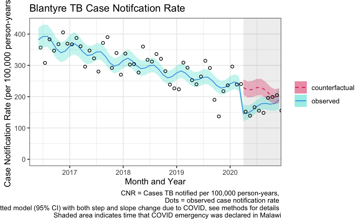
# Plot observed values and predictions
ggplot() +
geom_rect(aes(xmin=covid_date_m, xmax=dmy("31 Dec 2020"), ymin=-Inf, ymax=Inf), alpha=0.1) +
geom_line(aes(y=cnr_pred, x=seq, linetype="observed", color="observed"), data=plot_df %>% filter(c_fact==F)) +
geom_ribbon(aes(ymax=cnr_high, ymin=cnr_low, x=seq, fill="observed"), alpha=0.3, data=plot_df %>% filter(c_fact==F)) +
geom_line(aes(y=cnr_pred, x=seq, linetype="counterfactual", color="counterfactual"), data=plot_df %>% filter(c_fact==T)) +
geom_ribbon(aes(ymax=cnr_high, ymin=cnr_low, x=seq, fill="counterfactual"), alpha=0.3, data=plot_df %>% filter(c_fact==T)) +
  geom_point(aes(y=cnr_actual, x=month+days(15)), data=plot_df, shape=1) + # plot actual numbers on 15th each month
  #geom_vline(aes(xintercept=covid_date_m)) +
  scale_linetype_manual(name="legend",values=c("dashed","solid")) +
  scale_fill_manual(name="legend", values=c("#DE3163","#3FE0D0")) +
  scale_color_manual(name="legend", values=c("#DE3163","#4286f4")) +
  ylab("Case Notification Rate (per 100,000 person-years)") +
    xlab("Month and Year") +
   labs(title="Blantyre TB Case Notifcation Rate",
       caption="CNR = Cases TB notified per 100,000 person-years, \n Dots = observed case notification rate \n Line = fitted model (95% CI) with both step and slope change due to COVID, see methods for details \n Shaded area indicates time that COVID emergency was declared in Malawi") +
  coord_cartesian(xlim=c(dmy("01 April 2016"), dmy("31 Dec 2020")),ylim=c(0,430)) +
  scale_x_date(expand = c(0,0)) + 
  theme_bw()  %+replace%
    theme(legend.title = element_blank())

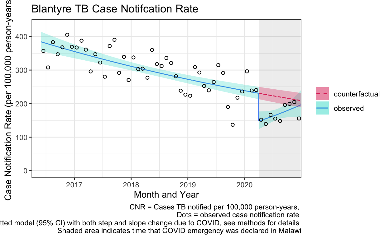
And some examples of predications from model

m1_nb_all %>% filter(month==dmy("01 March 2020") | month==dmy("01 April 2020")) %>% select(-month_num, -yq, -m, -pop, -value)

# A tibble: 3 x 13
  covid month      cases_actual cnr_actual cases_pred cnr_pred
  <int> <date>            <int>      <dbl>      <dbl>    <dbl>
1     0 2020-03-01          168       240.       163.     233.
2     0 2020-04-01           NA        NA        162.     231.
3     1 2020-04-01          107       152.       104.     148.
# … with 7 more variables: cases_low <dbl>, cases_high <dbl>,
#   cnr_low <dbl>, cnr_high <dbl>, cases_se <dbl>, cases_link <dbl>,
#   c_fact <lgl>

m1_nb_all %>% filter(month==dmy("01 Nov 2020") | month==dmy("01 Dec 2020")) %>% select(-month_num, -yq, -m, -pop, -value)

# A tibble: 4 x 13
  covid month      cases_actual cnr_actual cases_pred cnr_pred
  <int> <date>            <int>      <dbl>      <dbl>    <dbl>
1     0 2020-11-01           NA        NA        152.     214.
2     1 2020-11-01          146       205.       132.     185.
3     0 2020-12-01           NA        NA        151.     211.
4     1 2020-12-01          111       156.       136.     191.
# … with 7 more variables: cases_low <dbl>, cases_high <dbl>,
#   cnr_low <dbl>, cnr_high <dbl>, cases_se <dbl>, cases_link <dbl>,
#   c_fact <lgl>

Model checking

res1 <- residuals(m1_nb,type="deviance")
plot(all$month_num,res1,ylim=c(-5,10),pch=19,cex=0.7,col=grey(0.6),
     main="Residuals over time",ylab="Deviance residuals",xlab="Date")

# Further check for autocorrelation by examining the autocorrelation and
#   partial autocorrelation functions
acf(res1)

pacf(res1)

Use model to illustrate “missing cases” / missing CNR. Use parametric bootstrapping to get confidence intervals

# c_fact = FALSE (from April to December) is a modelled estimate (with a CI), BUT, the model estimate and the actual observed value (i.e. 505 cases) is identical.  So going to use this as a constant, without a distribution.

m1_nb_covidt <- m1_nb_all %>% filter(month>=covid_date_m) #only interested in time period after "COVID time"

#NB. This is covid_no when you just return the modelled cases (on the link scale 'cases_link'); the next function replaces cases_link with a distribution with mean 'cases_link' and st. dev 'st.error' of fir

covid_no <- m1_nb_covidt %>% filter(c_fact==T) %>%
  summarise(n_nocovid = sum(
    exp(
      cases_link
      )))

boot_fx <- function(df){
covid_yes <- df %>% filter(c_fact==F) %>%
  summarise(n_actual = sum(cases_actual))

covid_no <- df %>% filter(c_fact==T) %>%
  summarise(n_nocovid = sum(
    exp(
      as.numeric(pmap(list(cases_link,cases_se), function(mu, sd) rnorm(1, mu, sd))) 
      )))

abs_diff <- covid_no - covid_yes
rel_diff <- (covid_no - covid_yes) / covid_no

as.numeric(c(covid_yes,covid_no,abs_diff,rel_diff))
}

# run once to check
boot_fx(m1_nb_covidt) # col 1 = observed cases, col 2 = predicted under counterfactual, col 3 = abs difference, col 4 = rel diff (one replicate)

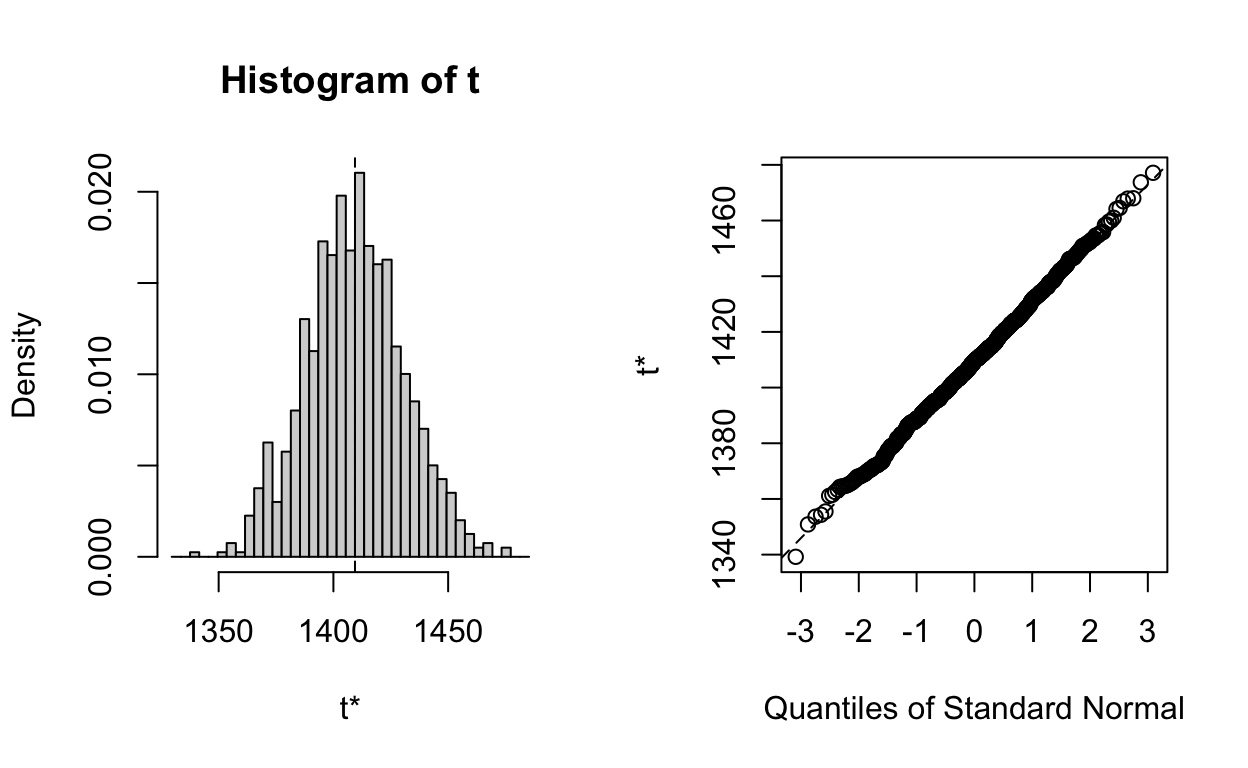
[1] 1075.0000000 1437.5813802  362.5813802    0.2522162

# now run 1000 times
x <- boot(m1_nb_covidt,boot_fx,R=1000,sim="parametric")

# Plot output for predicted number of cases under counterfactual no-COVID
plot(x, index=2)

sd_x <- c(sd(x$t[,1]),sd(x$t[,2]),sd(x$t[,3]),sd(x$t[,4])) # boot command output is a vector of estimate for worst / actual / averted

# Now generate estimates with CI (using point estimate from model (cases_pred) rather than mean of boot output, although should be v. similar)
table_fx <- function(df,sd){
  covid_yes <- df %>% filter(c_fact==F) %>%
  summarise(n_actual = sum(cases_actual)) %>%
    mutate(str=n_actual)
  
  covid_no <- df %>% filter(c_fact==T) %>%
  summarise(n = sum(
    exp(
      cases_link
      ))) %>%
    mutate(nhi = n + 1.96*sd[2],
            nlo = n - 1.96*sd[2]) %>%
    mutate(str = paste0(
      round(n,digits=0)," (",round(nlo,digits=0)," to ",round(nhi,digits=0),")"
    ))
  
  abs_diff <- tibble(covid_no$n - covid_yes) %>%
    rename(n=n_actual) %>%
    mutate(
    nhi = n + 1.96*sd[3],
    nlo = n - 1.96*sd[3]) %>%
  mutate(str = paste0(
      round(n,digits=0)," (",round(nlo,digits=0)," to ",round(nhi,digits=0),")"
  ))
  
  rel_diff <- tibble((covid_no$n - covid_yes) / covid_no$n) %>%
    rename(n=n_actual) %>%
    mutate(
    nhi = n + 1.96*sd[4],
    nlo = n - 1.96*sd[4]) %>%
  mutate(str = paste0(
      round(n,digits=3)," (",round(nlo,digits=3)," to ",round(nhi,digits=3),")"
  ))
  
  cbind(covid_yes$str, covid_no$str, abs_diff$str, rel_diff$str) %>% as_tibble() %>%
    rename(covid_yes=V1,
           covid_no=V2,
           rel.diff = V3,
           abs.diff = V4)
}

table_fx(m1_nb_covidt,sd_x) %>% gt()

covid_yes	covid_no	rel.diff	abs.diff
1075	1408 (1367 to 1450)	333 (292 to 375)	0.237 (0.214 to 0.259)

m1_nb_covidt %>% filter(c_fact==T) %>% summarise(mean=mean(cnr_pred))

# A tibble: 1 x 1
   mean
  <dbl>
1  221.

3. Now to break this down by demographics

Health centre, sex and HIV status. Cases rather than CNR, as don’t have denominators for health centre or HIV status

# Impute the small number of missing variables
tb_data_mids <- mice(
  data=tb_data,
  m=1, #just one imputation as missing data v. small
  method="pmm"
)

 iter imp variable
  1   1  sex  hiv
  2   1  sex  hiv
  3   1  sex  hiv
  4   1  sex  hiv
  5   1  sex  hiv

tb_data_imp <- complete(tb_data_mids, action="long") %>% select(-.imp, -.id) #complete data set

by <- tb_data_imp %>%
    group_by(month,sex,hiv,fac) %>%
    summarise(cases=n()) %>%
    ungroup() %>%
    mutate(covid = if_else(month >= covid_date_m, 1L,0L)) %>%
    arrange(month) %>%
    group_by(month) %>%
    mutate(month_num = cur_group_id()) %>%
    ungroup()

m2 <-glm.nb(cases ~ sex + hiv + fac + sex:hiv:fac + sex:hiv:fac:covid + sex:hiv:fac:month_num + sex:hiv:fac:covid:I(month_num-covid_month_num), data=by) 

tidy(m2, exp=T, conf.int = T) %>% gt()

term	estimate	std.error	statistic	p.value	conf.low	conf.high
(Intercept)	11.5682613	0.192838705	12.69592250	6.229160e-37	7.9042010	16.9111105
sexmale	1.4474150	0.100884418	3.66537463	2.469768e-04	1.1856677	1.7673495
hivpositive	2.4921744	0.109810004	8.31577778	9.115248e-17	2.0102265	3.0925538
facqech	1.4340115	0.100884422	3.57315552	3.527051e-04	1.1749379	1.7506146
sexfemale:hivnegative:fachc	1.0206506	0.217852134	0.09382613	9.252473e-01	0.6642900	1.5684400
sexmale:hivnegative:fachc	1.5151800	0.154147308	2.69569568	7.024181e-03	1.1205023	2.0493665
sexfemale:hivpositive:fachc	0.8914292	0.150287341	-0.76473002	4.444323e-01	0.6622342	1.1996924
sexmale:hivpositive:fachc	NA	NA	NA	NA	NA	NA
sexfemale:hivnegative:facqech	0.9832463	0.164035493	-0.10299973	9.179632e-01	0.7118945	1.3572887
sexmale:hivnegative:facqech	NA	NA	NA	NA	NA	NA
sexfemale:hivpositive:facqech	NA	NA	NA	NA	NA	NA
sexmale:hivpositive:facqech	NA	NA	NA	NA	NA	NA
sexfemale:hivnegative:fachc:covid	0.4991993	0.282092709	-2.46284264	1.378404e-02	0.2807735	0.8565982
sexmale:hivnegative:fachc:covid	0.6571969	0.190951350	-2.19831715	2.792651e-02	0.4502135	0.9550982
sexfemale:hivpositive:fachc:covid	0.6096585	0.247231918	-2.00158736	4.532913e-02	0.3715020	0.9785294
sexmale:hivpositive:fachc:covid	0.6480760	0.202645855	-2.14042027	3.232082e-02	0.4326924	0.9629001
sexfemale:hivnegative:facqech:covid	0.5421471	0.306924115	-1.99468824	4.607689e-02	0.2885525	0.9726948
sexmale:hivnegative:facqech:covid	0.6447441	0.241977617	-1.81381172	6.970672e-02	0.3965319	1.0275156
sexfemale:hivpositive:facqech:covid	0.6673820	0.197849197	-2.04394415	4.095906e-02	0.4495570	0.9840863
sexmale:hivpositive:facqech:covid	0.6994277	0.185914310	-1.92289071	5.449378e-02	0.4845232	1.0055719
sexfemale:hivnegative:fachc:month_num	1.0032003	0.003707896	0.86172439	3.888392e-01	0.9958843	1.0105793
sexmale:hivnegative:fachc:month_num	1.0047130	0.002900554	1.62106168	1.050044e-01	0.9991064	1.0103592
sexfemale:hivpositive:fachc:month_num	0.9880795	0.003237245	-3.70443120	2.118656e-04	0.9817517	0.9944184
sexmale:hivpositive:fachc:month_num	0.9895807	0.002805365	-3.73353915	1.888078e-04	0.9840929	0.9950830
sexfemale:hivnegative:facqech:month_num	0.9865843	0.003814012	-3.54128552	3.981824e-04	0.9791794	0.9939974
sexmale:hivnegative:facqech:month_num	0.9881350	0.003304539	-3.61199987	3.038447e-04	0.9817762	0.9945050
sexfemale:hivpositive:facqech:month_num	0.9903053	0.002799128	-3.48036450	5.007320e-04	0.9848125	0.9958134
sexmale:hivpositive:facqech:month_num	0.9849039	0.002658260	-5.72223395	1.051324e-08	0.9797209	0.9900946
sexfemale:hivnegative:fachc:covid:I(month_num - covid_month_num)	0.9726919	0.056988957	-0.48584754	6.270753e-01	0.8684701	1.0885607
sexmale:hivnegative:fachc:covid:I(month_num - covid_month_num)	0.9977264	0.036736922	-0.06195886	9.505956e-01	0.9277265	1.0730474
sexfemale:hivpositive:fachc:covid:I(month_num - covid_month_num)	1.0407859	0.047241179	0.84621354	3.974336e-01	0.9494280	1.1416900
sexmale:hivpositive:fachc:covid:I(month_num - covid_month_num)	1.0175961	0.039192492	0.44506076	6.562758e-01	0.9417458	1.0996888
sexfemale:hivnegative:facqech:covid:I(month_num - covid_month_num)	1.1008144	0.056097551	1.71220025	8.685977e-02	0.9858711	1.2324208
sexmale:hivnegative:facqech:covid:I(month_num - covid_month_num)	1.0945064	0.044228367	2.04175590	4.117575e-02	1.0037741	1.1951421
sexfemale:hivpositive:facqech:covid:I(month_num - covid_month_num)	1.0368200	0.037630942	0.96086734	3.366189e-01	0.9622314	1.1175599
sexmale:hivpositive:facqech:covid:I(month_num - covid_month_num)	1.0821023	0.034547361	2.28398582	2.237236e-02	1.0115490	1.1582752

coeffs2 <- tidy(m2, exp=T, conf.int = T)

Check model

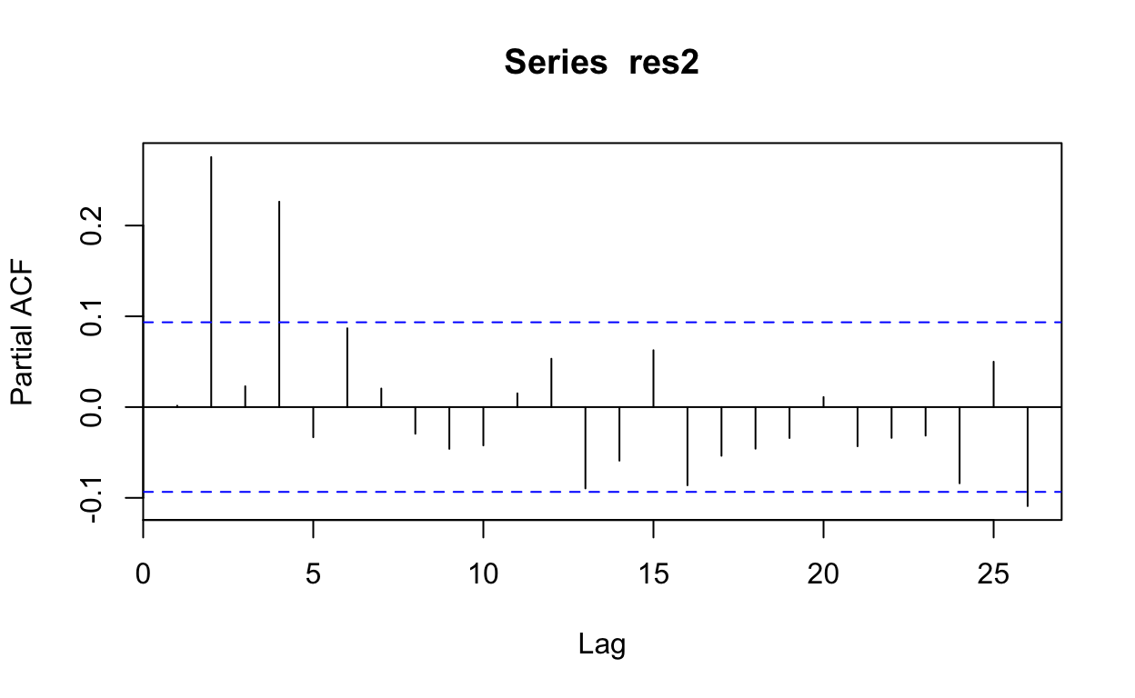
res2 <- residuals(m2,type="deviance")
plot(by$month_num,res2,ylim=c(-5,10),pch=19,cex=0.7,col=grey(0.6),
     main="Residuals over time",ylab="Deviance residuals",xlab="Date")

# Further check for autocorrelation by examining the autocorrelation and
#   partial autocorrelation functions
acf(res2)

pacf(res2)

Make predictions and plot them

m2_by <- model2pred_by(by,m2)
m2_by_continuous <- model2pred_by_continuous(by,m2)

# the below bit of code (and 'plot df' is a slightly hack-y way to make 'seq' correspond to real dates to be able to plot)
cTb <- m2_by_continuous %>% filter(c_fact==T) # creating a sequence of dates to match month_num (a continuous numerical value)
start_cTb <- min(cTb$month, na.rm=T)
end_cTb <- max(cTb$month, na.rm=T) + months(1) - days(1) # the end date needs to be the END of the month, not the start of the month
length_cTb <- cTb %>% nrow()
seq_cTb <- seq.Date(start_cTb,end_cTb,length.out = length_cTb) 

cFb <- m2_by_continuous %>% filter(c_fact==F)
start_cFb <- min(cFb$month, na.rm=T)
end_cFb <- max(cFb$month, na.rm=T) + months(1) - days(1)
length_cFb <- cFb %>% nrow()
seq_cFb <- seq.Date(start_cFb,end_cFb,length.out = length_cFb) 

seqb <- c(seq_cFb, seq_cTb)

plot_df_by <- m2_by_continuous %>% arrange(c_fact,month_num) %>% cbind(seqb) # "plot df" has month_num transformed to actual date


label_hc <- c( #labels for plot
  hc = "Health Centre",
  qech = "Queen Elizabeth Central Hospital"
)

label_hiv <- c( #labels for plot
  negative="HIV Negative",
  positive="HIV Positive"
)

ggplot() +
  geom_line(aes(y=cases_pred,x=seqb, color=sex), data=plot_df_by%>%filter(c_fact==F)) +
  geom_ribbon(aes(ymax=cases_high, ymin=cases_low, x=seqb, fill=sex), alpha=0.3, data=plot_df_by %>% filter(c_fact==F)) +
  geom_point(aes(y=cases_actual, x=month+days(15), color=sex), size=0.5, alpha=0.7, data=plot_df_by%>%filter(c_fact==F))+
  geom_vline(xintercept=covid_date_m, linetype="dotted") +
  scale_fill_manual(name="legend", values=c("#E58601","#B40F20")) +
  scale_color_manual(name="legend", values=c("#E58601","#B40F20")) +
  ylab("Number of TB cases notified per month") +
  xlab("Month and Year") +
  labs(title="",
       caption="Dots = observed number of cases \n Line = fitted model (95% CI) with both step and slope change due to COVID, see methods for details \n Vertical lines indicates time that COVID emergency was declared in Malawi") +
  facet_grid(hiv~fac, 
             labeller=labeller(
               fac=label_hc,
               hiv=label_hiv
             )) +
  theme_bw() %+replace%
    theme(legend.title = element_blank())

Use model to make predictions by number

# Point estimate of missing
m2_by %>% group_by(month,c_fact) %>% summarise(n=sum(cases_pred)) %>% filter(month>=covid_date_m) %>% group_by(c_fact) %>% summarise(n=sum(n)) 

# A tibble: 2 x 2
  c_fact     n
  <lgl>  <dbl>
1 FALSE  1075.
2 TRUE   1427.

y <- m2_by %>% group_by(month,c_fact) %>% summarise(n=sum(cases_pred)) %>% filter(month>=covid_date_m) %>% group_by(c_fact) %>% summarise(n=sum(n)) 
y[2,2] - y[1,2] 

         n
1 351.9844

# Boot-strappable function
m2_by_covidt <- m2_by %>% filter(month>=covid_date_m)

boot_fx_by <- function(df,var){
  var <- enquo(var)

  covid_yes <- df %>% 
    filter(c_fact==F) %>%
    group_by(!!var) %>%
    summarise(
      n=sum(
        cases_actual
      ))
 
  covid_no <- df %>%
    filter(c_fact==T) %>%
    group_by(!!var) %>%
    summarise(
      n=sum(
        cases_pred
      ))  
  
  abs_diff <- covid_no$n - covid_yes$n
  rel_diff <- (covid_no$n - covid_yes$n) / covid_no$n
  
  covid_yes %>% left_join(covid_no,by=quo_name(var)) %>% cbind(abs_diff) %>% cbind(rel_diff) %>%
    rename(covid_yes=n.x,
           covid_no=n.y)
}

# Run each of these once to have a look
boot_fx_by(m2_by_covidt,sex)

     sex covid_yes covid_no abs_diff  rel_diff
1 female       381 550.8405 169.8405 0.3083297
2   male       694 876.1896 182.1896 0.2079340

boot_fx_by(m2_by_covidt,hiv)

       hiv covid_yes covid_no abs_diff  rel_diff
1 negative       416 606.6919 190.6919 0.3143142
2 positive       659 820.3382 161.3382 0.1966728

boot_fx_by(m2_by_covidt,fac)

   fac covid_yes covid_no  abs_diff  rel_diff
1   hc       488 761.0615 273.06150 0.3587903
2 qech       587 665.9686  78.96858 0.1185770

# Annoyingly, I can't work out how to pass second variable within my function to "boot" (ie. can't add a var).
# Go back to original boot function

# Boot sex

male <- m2_by_covidt %>% filter(sex=="male")
female <- m2_by_covidt %>% filter(sex=="female")
hc <- m2_by_covidt %>% filter(fac=="hc")
qech <- m2_by_covidt %>% filter(fac=="qech")
hivpos <- m2_by_covidt %>% filter(hiv=="positive")
hivneg <- m2_by_covidt %>% filter(hiv=="negative")



# Then boot each one
male_res <- boot(male,boot_fx,R=1000,sim="parametric")
female_res <- boot(female,boot_fx,R=1000,sim="parametric")
hc_res <- boot(hc,boot_fx,R=1000,sim="parametric")
qech_res <- boot(qech,boot_fx,R=1000,sim="parametric")
hivpos_res <- boot(hivpos,boot_fx,R=1000,sim="parametric")
hivneg_res <- boot(hivneg,boot_fx,R=1000,sim="parametric")
all_res <- boot(m2_by_covidt, boot_fx, R=1000, sim="parametric")

#Get st. dev
boot_sd <- function(var){
  c(sd(var$t[,1]),sd(var$t[,2]),sd(var$t[,3]),sd(var$t[,4]))
}

sd_male <- boot_sd(male_res)
sd_female <- boot_sd(female_res)
sd_hc <- boot_sd(hc_res)
sd_qech <- boot_sd(qech_res)
sd_hivpos <- boot_sd(hivpos_res)
sd_hivneg <- boot_sd(hivneg_res)
sd_all <- boot_sd(all_res)

table_fx_2 <- function(df,df_sd){ #not using boot function results, as get the point estimate direct from model; but using boot st. devs
  covid_yes <- df %>% filter(c_fact==F) %>%
  summarise(n_actual = sum(cases_actual)) %>%
    mutate(str=n_actual)
  
  covid_no <- df %>% filter(c_fact==T) %>%
  summarise(n = sum(
    exp(
      cases_link
      ))) %>%
    mutate(nhi = n + 1.96*df_sd[2],
            nlo = n - 1.96*df_sd[2]) %>%
    mutate(str = paste0(
      round(n,digits=0)," (",round(nlo,digits=0)," to ",round(nhi,digits=0),")"
    ))
  
  abs_diff <- tibble(covid_no$n - covid_yes) %>%
    rename(n=n_actual) %>%
    mutate(
    nhi = n + 1.96*df_sd[3],
    nlo = n - 1.96*df_sd[3]) %>%
  mutate(str = paste0(
      round(n,digits=0)," (",round(nlo,digits=0)," to ",round(nhi,digits=0),")"
  ))
  
  rel_diff <- tibble((covid_no$n - covid_yes) / covid_no$n) %>%
    rename(n=n_actual) %>%
    mutate(
    nhi = n + 1.96*df_sd[4],
    nlo = n - 1.96*df_sd[4]) %>%
  mutate(str = paste0(
      round(n,digits=3)," (",round(nlo,digits=3)," to ",round(nhi,digits=3),")"
  ))
  
  cbind(covid_yes$str, covid_no$str, abs_diff$str, rel_diff$str) %>% as_tibble() %>%
    rename(covid_yes=V1,
           covid_no=V2,
           abs.diff = V3,
          rel.diff = V4)
}

table_fx_2(male,sd_male) %>%
  bind_rows(table_fx_2(female,sd_female)) %>%
  bind_rows(table_fx_2(hc,sd_hc)) %>%
  bind_rows(table_fx_2(qech,sd_qech)) %>%
  bind_rows(table_fx_2(hivpos,sd_hivpos)) %>%
  bind_rows(table_fx_2(hivneg,sd_hivneg)) %>%
  cbind(c("male","female","hc","qech","hivpos","hivneg")) %>% 
  rename(group = `c(\"male\", \"female\", \"hc\", \"qech\", \"hivpos\", \"hivneg\")`) %>%
  select(group,everything()) %>%
  gt()

group	covid_yes	covid_no	abs.diff	rel.diff
male	694	876 (850 to 902)	182 (156 to 208)	0.208 (0.184 to 0.231)
female	381	551 (532 to 570)	170 (151 to 189)	0.308 (0.285 to 0.332)
hc	488	761 (736 to 786)	273 (248 to 298)	0.359 (0.338 to 0.38)
qech	587	666 (645 to 687)	79 (58 to 100)	0.119 (0.091 to 0.146)
hivpos	659	820 (796 to 844)	161 (137 to 185)	0.197 (0.173 to 0.22)
hivneg	416	607 (585 to 629)	191 (169 to 213)	0.314 (0.29 to 0.339)

# Table for everyone
table_fx_2(m2_by_covidt,sd_all) %>% gt()

covid_yes	covid_no	abs.diff	rel.diff
1075	1427 (1394 to 1460)	352 (319 to 385)	0.247 (0.23 to 0.264)

Sensitivity analysis

# Harmonics for seasons
sens1 <- glm.nb(cases ~ offset(log(pop)) + covid*month_num + harmonic(month_num,2,12), all)  # have to use month_num here as I can't get 'harmonic' to work sensibly with dates

s1_all <- model2pred_pop(all,sens1)

plot_all_fx <- function(df){
ggplot() +
geom_rect(aes(xmin=covid_date_m, xmax=dmy("15 Dec 2020"), ymin=-Inf, ymax=Inf), alpha=0.1) +
geom_line(aes(y=cnr_pred, x=month, linetype="observed", color="observed"), data=df %>% filter(c_fact==F)) +
geom_ribbon(aes(ymax=cnr_high, ymin=cnr_low, x=month, fill="observed"), alpha=0.3, data=df %>% filter(c_fact==F)) +
geom_line(aes(y=cnr_pred, x=month, linetype="counterfactual", color="counterfactual"), data=df %>% filter(c_fact==T)) +
geom_ribbon(aes(ymax=cnr_high, ymin=cnr_low, x=month, fill="counterfactual"), alpha=0.3, data=df %>% filter(c_fact==T)) +
  geom_point(aes(y=cnr_actual, x=month+days(15)), data=plot_df, shape=1) + # plot actual numbers on 15th each month
  #geom_vline(aes(xintercept=covid_date_m)) +
  scale_linetype_manual(name="legend",values=c("dashed","solid")) +
  scale_fill_manual(name="legend", values=c("#DE3163","#3FE0D0")) +
  scale_color_manual(name="legend", values=c("#DE3163","#4286f4")) +
  ylab("Case Notification Rate (per 100,000 person-years)") +
    xlab("Month and Year") +
   labs(title="Blantyre TB Case Notifcation Rate",
       caption="CNR = Cases TB notified per 100,000 person-years, \n Dots = observed case notification rate \n Line = fitted model (95% CI) with both step and slope change due to COVID, see methods for details \n Shaded area indicates time that COVID emergency was declared in Malawi") +
  coord_cartesian(xlim=c(dmy("01 April 2016"), dmy("15 Dec 2020")),ylim=c(0,430)) +
  scale_x_date(expand = c(0,0)) + 
  theme_bw()  %+replace%
    theme(legend.title = element_blank())
}


plot_all_fx(s1_all)

s1_covidt <- s1_all %>% filter(month>=covid_date_m) 
boot_fx(s1_covidt)

[1] 1075.0000000 1424.9239975  349.9239975    0.2455738

est_s1 <- boot(s1_covidt,boot_fx,R=100,sim="parametric")
sd_s1 <- c(sd(est_s1$t[,1]),sd(est_s1$t[,2]),sd(est_s1$t[,3]),sd(est_s1$t[,4])) # boot command output is a vector of estimate for worst / actual / averted

table_fx(s1_covidt,sd_s1)

# A tibble: 1 x 4
  covid_yes covid_no            rel.diff         abs.diff             
  <chr>     <chr>               <chr>            <chr>                
1 1075      1387 (1335 to 1438) 312 (260 to 363) 0.225 (0.196 to 0.25…

table_fx(m1_nb_covidt,sd_x)

# A tibble: 1 x 4
  covid_yes covid_no            rel.diff         abs.diff             
  <chr>     <chr>               <chr>            <chr>                
1 1075      1408 (1367 to 1450) 333 (292 to 375) 0.237 (0.214 to 0.25…

m1_nb$aic

[1] 519.1786

sens1$aic #actually a little higher, no serious difference

[1] 523.2373

333/ all %>% filter(month>=dmy("01 April 2020")) %>% summarise(m=median(pop)) *100000

         m
1 39.16637